- Introduction to Aggs
- Horizontal Aggs
- Mixing Agg and base table to produce a single value
- Mixing Agg and base table to produce a single value
- Accordion Aggs (this article)
- Variable grain aggs in a single table for extra flexibility
- Variable grain aggs in a single table for extra flexibility
- Filtered Aggs
- Using Composite Models to keep recent data in memory, and older data in the source to optimise the model size
- Using Composite Models to keep recent data in memory, and older data in the source to optimise the model size
- Incremental Aggs
- A smart way to update Agg tables to optimise refresh time
- A smart way to update Agg tables to optimise refresh time
- Shadow Models
- Create manual DUAL mode tables to work around some current limitations of Agg Awareness
Introduction
Part III in this series looks at another time-based aggregation technique you can add to models. The basic idea of any aggregation table is to generate a summary table the engine can use produce the same result it might otherwise obtain from a much larger table.
It will always be slower to scan 100 rows of data in a table, compared with scanning a handful of preprocessed rows in an Agg table. Remember the benefit of an agg table is not just faster query times. The server resource freed up by speedier queries becomes available to other concurrent query demand – so can exponentially pay off on busy systems.
The question is, what is the most effective aggregation strategy for any given model. Yes, it is possible to have too many aggregation tables in a model. There is a point where the management overhead starts to outweigh the performance gains, and each aggregation table you add increases the size of your model. If the combined physical size of your aggregations ends up being larger than the raw data, you may have gone overboard.
So, care should be taken when designing an aggregation table strategy to ensure the overall benefits outweigh the potential downsides of additional tables.
There are different ways to generate and use aggregate raw data. This series is looking at a few I have come across and liked enough to share. The last article looked at Horizontal Aggs. This article is going to introduce the idea of Accordion Aggs, which aside from anything else, has a cooler name. Someone did suggest I may need to explain what an accordion is to a younger audience. I think Wikipedia can provide a much better explanation than I can.
Accordion Aggs
Accordion Aggs is a technique primarily for summarising a Time dimension, although potentially could be used for other dimension types.
A common time-based aggregation strategy is to generate an Agg table based on calendar months and to have a separate aggregation table based on weekly periods.
A calendar month aggregation table can be used to produce results for a single month, a series of months or years.
A week-based aggregation table can be used to quickly produce results based on a single week or set of weeks (last 13 weeks, 454, week on week comparisons etc.)
On the surface, these two methods to summarise data appear to be incompatible as they do not vertically align. What I mean by vertically align, is while you can use a calendar month aggregation table to generate accurate results for calendar years safely, you cannot use a week-based aggregation table to generate month or year values. The start and end dates for a week, month and year periods will rarely align.
A week based aggregation table will summarise raw data into even blocks of 7-days. Often the value chosen as the aggregation key will be the start (or end) date for the seven days. The day of the week used as the start (or end) will match your organisational reporting preferences. The table will have a consistent cadence/rhythm to the values stored in the time-key column.
Likewise, a calendar month based aggregation table will summarize raw data into mostly even blocks that begin on the first of each calendar month. The unique values in the time-key column of this table get evenly spaced.
Accordion Aggs combine both a week and calendar month based aggs into a single table.
How does this work?
Consider a simplified set of raw data that starts on Friday, 1 March 2019. The data-set has a single row for every day (no gaps or overlaps), and the value for each day is always 10.

A week-based aggregation table over this data will always carry the value of 70 in the sum-of column. The calendar month version will carry an amount 10x the number of days in that specific month.
An accordion agg table does not use even spacing between values in the time column. Accordion aggs combine summarization boundary values for both week and month groupings to a single column but can still be used to generate values for any combination of full weeks, months or years from a single table.
An expanded view of our raw table shows data from Friday 1 March 2019 into the following April. You will notice I have added a [Boundary] column to the left-hand table to display an X on any row that happens to coincide with the start of a calendar month or a Sunday based week. The [Boundary] column shown here is only needed to explain visually. You do not need to add this column to your raw data in practice.
The only [Date] values added to the Accordion Agg table on the left are those from rows with an X. The [Sum of Value] column shows a number relevant to how much gets compressed into each row.

This example shows 44 rows from the base table can be represented using only eight rows in an accordion agg table. The accordion agg table is over 5x smaller so could potentially produce a value 5x faster than the same query using the base table.
If you want to show a sum of [Value] for March 2019, the following six rows from the accordion table can get used. The combined total of these rows should be 310, which will be the same if 31 rows get scanned from the base table. It will be the same story for other months (and years).

Now let’s look at which rows are needed to produce a value for the week starting Sunday 31 March.

You can see this week-based period is broken up over two rows because it straddles the start of a calendar month. This extra row doesn’t matter as the result is still correct. Most weeks will only need a single row, but occasionally this calculation may need to use two. This extra row still represents a decent saving compared with the same calculation running over the base table.
Agg Awareness
This technique is compatible with the Power BI Aggregation Awareness feature, so you can incorporate Accordion Aggs into your model without needing to write explicit DAX to take advantage of them. The technique also works very well with the row-based Time Intelligence approach, so you can also benefit from horizontal fusion.
The beauty of this technique is you don’t have to make your calculations aware of the irregular boundaries used by the Accordion Agg. This inconsistency resolves itself naturally through filters. By this, I mean – if you want to use the Accordion Agg table to show a value for March 2019, you don’t need first to work out what the specific Accordion boundary dates are. You apply a filter over the Accordion table for all 31 days that belong to March 2019. Six of those days will return a value, while 25 will harmlessly return nothing.
Selecting a month column in a calendar table, or making a month based selection from a row-based Time Intelligence table should end up applying day-level filtering through natural relationships and end up selecting the appropriate values from the Accordion Agg table.
One challenge is the agg table should not resolve filters placed on specific days. If a user places a filter on just 1 April 2019 in a calendar table, this value should only come from the base table (or day based agg table), rather than an accordion table. This caution is also valid if you have week or calendar month based agg tables in your model
Generating Accordion Agg tables
So far, we have covered the theory, but how do you go about generating an Accordion Agg table. It’s not too tricky, and I show here an approach using T-SQL.
The first step is to generate a combined list of boundary dates for each week and month period. I use the following:
	SELECT
		ROW_NUMBER() OVER (ORDER BY DateKey ASC) AS Row# ,
		[DateKey]
	INTO #Boundaries
	FROM [dim].[Date]
	WHERE
		WEEKDAY = 1 OR DAY([DateKey]) = 1

The #Boundaries temp table can be joined back to itself as follows to generate a set of accordion friendly time ranges.
	SELECT
		B.DateKey AS StartDate ,
		A.DateKey AS EndDate
	FROM #Boundaries AS A
		INNER JOIN #Boundaries AS B
			ON A.Row# = B.Row# + 1

The last block of code can be joined as a derived table in a GROUP BY statement over your FACT table to generate the new Accordion table.
	SELECT
		Boundaries.StartDate
		,[DeviceID]
		,[OperatingSystemID]
		,[OperatingSystemVersionID]
		,[GeographyID]
		,SUM([Quantity_ThisYear]) AS [Quantity_ThisYear]
		,SUM([Quantity_LastYear]) AS [Quantity_LastYear]
	INTO [fact].[MyEvents_AGG_Accordion]
	FROM [fact].[MyEvents] AS F
		INNER JOIN (
			SELECT
				B.DateKey AS StartDate ,
				A.DateKey AS EndDate
			FROM #Boundaries AS A
				INNER JOIN #Boundaries AS B
			ON A.Row# = B.Row# + 1
			) AS Boundaries
		ON  F.DateKey >= Boundaries.StartDate
		AND F.DateKey <  Boundaries.EndDate
	GROUP BY
		Boundaries.StartDate
		,[DeviceID]
		,[OperatingSystemID]
		,[OperatingSystemVersionID]
		,[GeographyID]
The example shown here was run over an 8.3 Billion row FACT table spanning two years. The Accordion Agg table generated by this statement ended up with only 2.5 Million rows.
In this model, I also have some other non-accordion aggregation tables for both week and calendar month that otherwise share the same dimensions.
You can see from the table below, the number of rows in the Accordion Agg table was slightly smaller than the week and month combined. The reason for this is some weeks/months share the same date, so there is a slight gain in compression.
| Table | Rows |
|---|---|
| Base Table | 8,231,630,715 |
| Pure Week Agg | 2,206,251 |
| Pure Month Agg | 628,175 |
| Accordion Agg | 2,558,871 |
If you are primarily reporting on Calendar months, you should opt for the much smaller Month table – but for visuals that mix and match week/month periods, the Accordion agg table is a pretty good candidate.
The Practical
The following is an example where I applied this technique to a large dataset. My raw data table has over 50 billion rows of data and sits in an Azure SQL DW database scaled to 400DTU. The data is telemetry events spanning two years. I also create a ‘FACT.MyEvents’ table that summarises the raw data down to an 8.3 billion row table. This table has links to six dimension tables (including time) in the same data source.
I then create a Power BI Desktop composite model which includes the 8.3 billion row ‘FACT.MyEvents’ table, but leaves it in Direct Query mode.
I then import an Accordion agg version of this table into the PBIX model. The model contains a set of Dimension tables grouped in box (1) which all use Dual storage mode.
The table at (2) is the Accordion Agg table, that has relationships to Date, Device and Geography. This table uses import storage mode.
Finally, the FACT table at (3) is the 8.3 billion row Direct Query base table. There is a measure on that does a SUM over the Quantity_ThisYear column

The next part was to create a simple table visual on a Power BI report canvas using some week and month based periods from the row-based Time Intelligence table (dim TimeIntelligence).

The query timings for a model that includes the Accordion Agg table get shown below. The query took 47ms to produce a value, and there are <matchFound> events showing the Accordion Agg table was used instead of the base table.

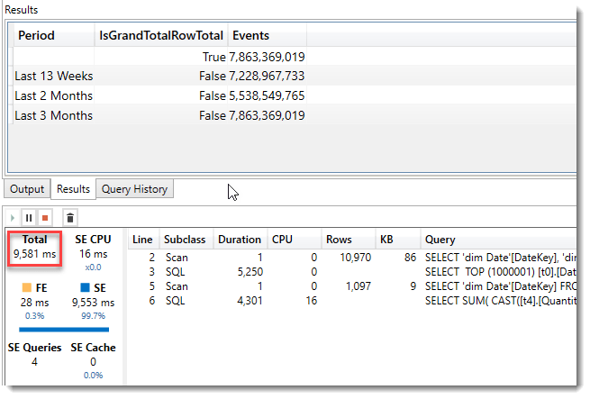
The results for the same query run on a version of the model that doesn’t have the Accordion Agg table get shown below. This time the query took 9.5 seconds (due to escaping out to a Direct Query table). Still, importantly, the values shown in the resultset are identical to the query in the model using the Accordion Agg.
I would expect any model that takes advantage of aggregations to outperform one without, especially when Direct Query is involved with large tables. What this example shows is you can mix and match variable grains within a dimension like this and still get the speed benefits without sacrificing accuracy.
Summary
As with other Aggregation techniques, there are pros and cons. Some of the advantages of Accordion Aggs is the ability to simplify models where reports mix the use of different periods that don’t initially appear to align.
The main disadvantage of this technique is you have to be careful to make sure a user can’t select a single day from a calendar table and assume the results they see are for that specific date, rather than for a more extended period. Explicit DAX can be added to measures to help return BLANK() if certain filters get used.
It might be a good fit for your model. Worth considering and as always, please feel free to reach out if you have questions or feedback relating to this.
Next up, Filtered Aggs.